4.6. Measuring dief@t at Different Answer Completeness Percentages

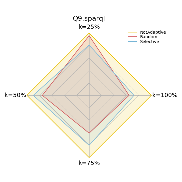
Experiment 2 in [1] compares the performance of the three variants of nLDE when producing different answer completeness percentages (25%, 50%, 75%, 100%) using dief@k.

The method diefpy.continuous_efficiency_with_diefk computes the dief@k metric for the previously mentioned answer completeness percentages.

import diefpy

COLORS = ["#ECC30B", "#D56062", "#84BCDA"]

# Load the answer trace file with the query traces from FigShare.
traces = diefpy.load_trace("https://ndownloader.figshare.com/files/9625852")

# Compute dief@k for 25%, 50%, 75%, and 100% answer completeness
exp2 = diefpy.continuous_efficiency_with_diefk(traces)

Create radar plot to compare the performance of the approaches with dief@k at different answer completeness percentages (25%, 50%, 75%, 100%). Plot interpretation: Lower is better.

diefpy.plot_continuous_efficiency_with_diefk(exp2, 'Q9.sparql', COLORS).show()

Conclusion: For Q9.sparql, the variants nLDE Random and Not Adaptive exhibit similar values of dief@k while producing the first 25% of the answers. However, when looking at dief@k at 100%, we can conclude that once nlDE Random starts producing answers, it produces all the answers at a faster rate. This can be observed in the answer trace plot, where the trace for nLDE Random (red line) has a higher slope over time than the other approaches.